Citation
These tutorials are a companion to:
Download the PDFPrerau MJ, Bianchi MT, Brown RE, Ellenbogen JM, Patrick PL. Sleep Neurophysiological Dynamics Through the Lens of Multitaper Spectral Analysis. Physiology (Bethesda). 2017 Jan;32(1):60-92. Review. doi: 10.1152/physiol.00062.2015 PubMed PMID: 27927806.
Code
Get the multitaper code for Matlab or PythonContents
- Tutorial: Learn about multitaper for spectral analysis of sleep EEG
- Spectral Scoring Manual: A guide for identify sleep patterns in the spectrogram
- Understanding and Setting Multitaper Parameters
- A Procedure for Setting Multitaper Parameters
- Multitaper Parameter Calculator
- Beyond Multitaper: The DYNAM-O Toolbox
Tutorial: Move Beyond the Hypnogram
In this set of online interactive tutorials, we will explain the theory of spectral estimation and demonstrate how a technique called multitaper spectral analysis can create clear, vibrant pictures of brain dynamics during sleep — rich with information beyond what can be seen in traditional clinical hypnogram analyses.
OverviewSleep is a continuous, dynamic neural process involving the complex interaction of many different networks within the brain. Long-standing clinical practice, however, breaks up sleep into discrete sleep stages through time-consuming, subjective, visual inspection of 30-second segments of electroencephalogram (EEG) data. As a result, vital information about brain activity is lost. Multitaper spectral analysis is therefore a powerful tool for finding new insights into the physiological mechanisms underlying sleep and for developing new ways of diagnosing and tracking sleep and diagnosing related disorders.
Part 1: An Introduction to Spectral Analysis
In Part 1 of this tutorial you will be introduced to spectral estimation, a powerful mathematical tool for analysis of neural oscillations present in the EEG. You will learn the history of characterizing the sleep EEG and why spectral estimation provides an objective, flexible, high-resolution alternative to traditional sleep staging.
Part 2: Methods of Spectral Estimation
In Part 2 of this tutorial you will learn the theory behind spectral estimation and common problems that occur when it is not applied in a principled manner. You will then learn about multitaper spectral analysis, a method of spectral estimation that greatly reduces the inaccuracy and noise present in other approaches. Finally, you will learn how to estimate the multitaper spectrogram in a principled manner, based on assumptions about the data you are studying.
Part 3: Characterizing Sleep with the Multitaper Spectrogram
In Part 3 of this tutorial you will learn how to apply the multitaper spectrogram to the analysis of sleep EEG data. You will learn the different spectral motifs that are hallmarks of the major sleep stages, as well as the spectral signatures of microevents such as spindles and K-complexes. With this knowledge, you should be able to characterize the dynamics and architecture of an entire night of sleep from the multitaper sleep EEG spectrogram alone. You will then learn about potential clinical and experimental applications for the use of the multitaper spectrogram.
Coding Exercise: Implementing Multitaper in Matlab
In this video, we go over an example implementation of the multitaper spectrogram in Matlab. To follow along, download the teaching version of multitaper_spectrogram.m for MATLAB here.
For research, make sure to use our GitHub code repository, which provides a more efficient implementation for deployment.
Spectral Scoring Manual
In order to facilitate sleep scoring using multitaper spectral analysis, in clinical practice we have developed a short Spectral Scoring Manual that provides a good overview of the principles of described in the tutorial above.
Download the Spectral Scoring Manual PDF
Understanding Multitaper Parameters
In multitaper spectral estimation, we define the properties of the spectrogram based on several parameters: Δf, N, TW, and L. In this section we will walk you through each of the parameters explaining what they mean and how to decide on what values to use.
Before anything else, YOU MUST THINK CRITICALLY ABOUT YOUR DATA. It is deeply important to understand WHY you are choosing a given set of parameters, what the assumptions underlying the data are, and the goals of your specific analysis. This guide will help you to make those decisions in a principled manner.
The Spectral Resolution (Δf)
This parameter defines the bandwidth (in Hz) of the main lobe in the spectral estimate, which controls the minimum distance between peaks that can be resolved. The main lobe of the spectral estimate can be thought of as blurring everything within it together, such that any structure within the spectral estimate cannot be seen. That means that any oscillations that are closer to each other than Δf will appear as a single mode within the spectrum.

We can illustrate the effect of Δf directly using simulated data that combines sinusoids at 10Hz and 12Hz. Since the difference between these oscillators is 2Hz, we should not be able to see them as separate oscillations when Δf is 2Hz or larger. In the figure below, we compute the multitaper spectrogram with estimators with varying spectral resolutions. On the top row, we can see the window spectra which show the size of the main lobe changing as we alter the spectral resolution. The bottom row shows the true/ideal spectrum (vertical lines at 10Hz and 12Hz) and the resulting multitaper estimate for each Δf. Technically, we can think of window spectra as being the shape that is convolved with each observed oscillation, acting like a smoothing window. Therefore, we only see two distinct peaks when Δf is less than the peak separation, which in this case is 2Hz.

In practice, it is vital to understand the oscillation structure of your data, and set the spectral resolution to be smaller than the minimum frequency distance between known oscillators. If you set Δf too large, you will merge multiple oscillator spectral peaks together in the estimate and not be able to resolve their individual properties. However, if you set Δf too small, you will reduce the number of tapers being used in the estimate, leading to a noisier estimate.
Frequency Bin Width vs. Spectral Resolution
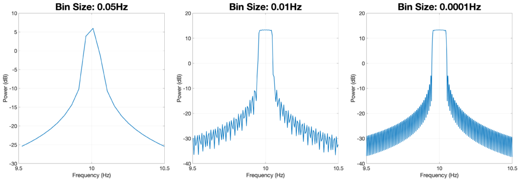
Spectral resolution is NOT the same as the width of the frequency bins! The width of the frequency bins at which a spectrum or spectrogram is computed is defined by the number of points in the FFT computation (NFFT) and the sampling rate. Therefore, the density of points within the estimated spectrum has nothing to do with the spectral resolution, which is the size of the main lobe bandwidth, Δf. Increasing the NFFT beyond the length of the data in your segment will zero-pad the data. Zero-padding has the effect of providing interpolation in the spectrum but will NOT improve the estimator.
In the example above, there are three spectra, all with the same spectral resolution but with different amounts of zero-padding (NFFT). Increasing the NFFT decreases the bin size and improves the interpolation used to create the spectral estimate, but the main lobe width remains unchanged.
Spectral Window Size (N)
The spectral window size (N) is the length of the data segment in seconds that is used to compute each spectrum. This parameter is very important because it reflects the stationary assumptions in your data. Spectrograms visualize the dynamics of data by breaking it up into many small windows and computing the spectrum within each window. The choice of window size imposes the assumption that the data spectral properties within each window are stationary (do not change). Therefore, it is important to understand the rate at which you expect your data to change over time and choose an N that reflects those dynamics.
Time Half-Bandwidth Product (TW)
The time half-bandwidth product (TW or sometimes NW) is defined literally as:
TW = (time: window size (N)) * (one-half) * (bandwidth: spectral resolution (Δf)) = N*(1/2)*Δf
The time half-bandwidth product controls the trade-off between frequency resolution and variance reduction. A higher TW increases the number of tapers used, which helps in reducing the variance of the spectral estimate but at the cost of lower frequency resolution. In practice, you first decide on N and Δf, which then helps you to define TW.
Number of Tapers (L)
The number of tapers, L, typically is defined as
L ≪ ⌊2TW − 1⌋
which means that L is selected to be much less than the floor (rounded down) of the quantity (2TW – 1). More tapers help in averaging out the noise, leading to a less noisy spectral estimate. However, using too many tapers can cause spectral leakage and should be avoided, even if the result looks cleaner. In practice, when data windows are short, we settle for L = ⌊2TW − 1⌋.
If your data assumptions are such that you can only use 1 taper to achieved the desired spectral resolution, you are not gaining anything from the multitaper method. Therefore, you should use a traditional single-taper spectrogram instead, using a Hann or other window depending on your application.
Reducing Variance: Trade-offs in Resolution
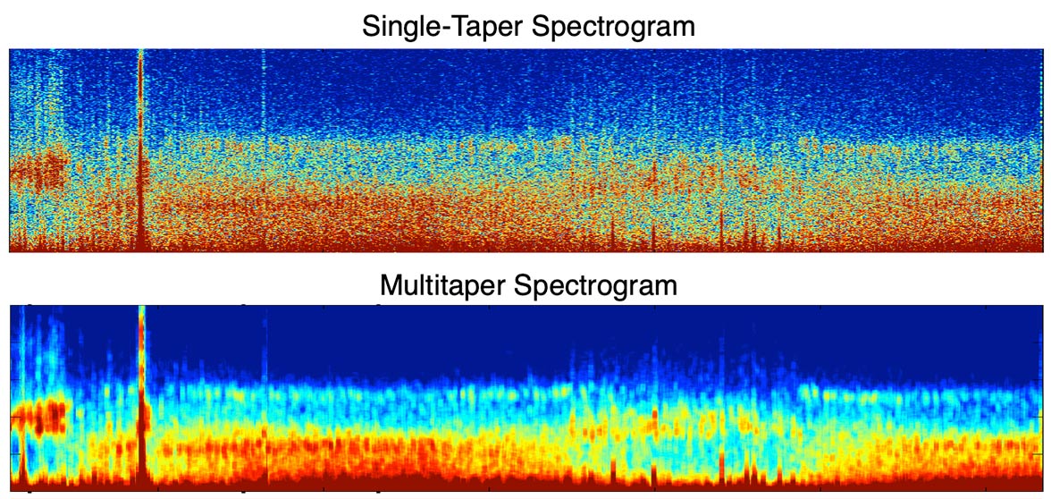
The chief benefit of the multitaper method is that it can reduce estimate variance (noise) through averaging across multiple tapers. Therefore, it is good to use as many tapers as you can within the limits of your data assumptions.
Given that L (number of tapers) is limited by TW (time half-bandwidth product), increasing TW will increase the upper bound of L. Since TW = NΔf/2, to increase TW, you can have a larger window size (N) and/or spectral resolution (Δf). This means that in order to have a less noisy estimate, you will have reduce your ability to look at differences in changes over time (by using a larger N), and/or your ability to distinguish close frequencies.

The example above illustrates this principle for a segment of sleep EEG during sleep onset. In this case, we are fixing the temporal resolution (N) to 30s, but losing the spectral resolution (increasing the value of Δf). We can then observe how the resulting spectrogram smooths out as we lose the distinctiveness of oscillations.
How to decide on this trade-off is a judgement call that should be based on the specific analyses you wish to perform and the data quality you are dealing with. For example, if you are looking at slow trends in a broad power band, you may be able to get away with a lower temporal/spectral resolution. However, if you are looking at short time-frequency peaks, such as spindles, which last only a few seconds and are band-limited in frequency, you may not be able to compromise in either dimension. By thinking critically about your data, you can come to a good compromise that provides a low-noise estimate that does not violate any major assumptions underlying the system you are studying.
A Procedure for Setting Multitaper Parameters
As stated above, the first step is that YOU MUST THINK CRITICALLY ABOUT YOUR DATA. There is no one-size-fits all parameter set that works on all data. This is a simple set of proposed steps that can help you to think through the assumptions that you will be imposing on your estimator and your analyses.
- How separated are the oscillations in the data?
- Set the desired frequency resolution Δf, based on the oscillatory structure of the data, such that it is less than the minimum frequency gap between known oscillations.
- How quickly is the spectral content changing?
- Set the window size N by determining the length of time over which the signal is assumed to be stationary.
- How noisy are your data?
- The noisier your data are, the more you will benefit by additional tapers, which reduce the estimate variance. This means a trade-off between variance, spectral resolution, and temporal resolution.
- How much spectral/temporal resolution can you afford to lose while maintaining valid assumptions about your data?
- Compute the taper parameters
- Compute the time-half-bandwidth product as TW = NΔf/2
- Compute the number of tapers as L ≪ ⌊2TW − 1⌋
- Note: In practice, given a small N and Δf, we set L = ⌊2TW − 1⌋
- If L = 1, then consider using a standard Hann single-taper spectrum.
Multitaper Spectral Parameter Calculator
Use this calculator to help you compute parameters for the multitaper spectrogram to fit a given specific application. Enter in pairs of parameters (N and TW, N and Δf, Δf and TW) and compute the missing values. Read the sections above for a detailed explanation of parameters.
MULTITAPER SPECTROGRAM PARAMETER CALCULATOR
Beyond Multitaper: The DYNAM-O Toolbox
Multitaper spectral analysis is but one of many powerful techniques for the analysis of time-varying data. Beyond other spectral estimators, state-space models, and other approaches, we can also think of the multitaper spectrogram not as the end result of the analysis, but rather as the input to other procedures. To these ends, we have developed the DYNAM-O (dynamic oscillation) toolbox, which extracts tens of thousands of time-frequency peaks from the spectrogram to study transient EEG oscillations.
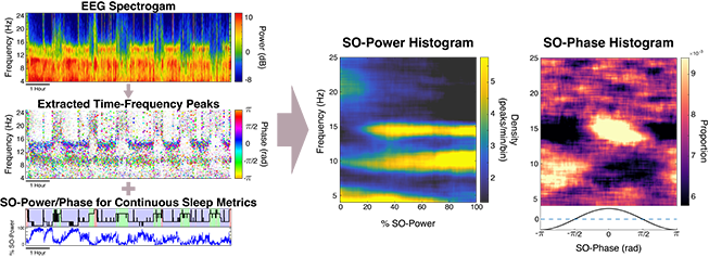
Using this approach, we are able to create fingerprint-like representations of brain state during sleep which appear to be highly individualized yet robust across days, months, and even over multiple years.