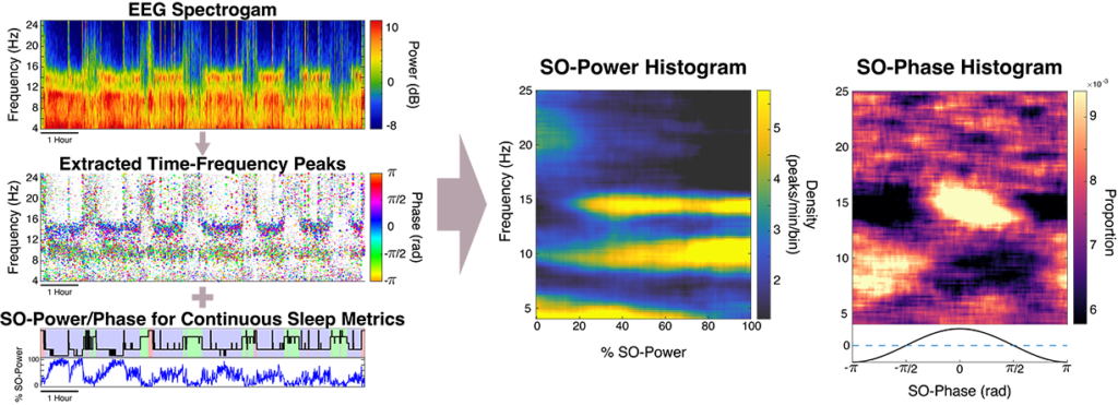
Transient Oscillation Dynamics with DYNAM-O

The DYNAM-O toolbox can be used to identify time-frequency peaks (TF-peaks) in the time-frequency topography of the EEG, then create two-dimensional histogram visualizations of TF-peak activity across continua of sleep-depth and cortical up/down state timing.

Citation

Please cite the following paper when using this package:

Patrick A Stokes, Preetish Rath, Thomas Possidente, Mingjian He, Shaun Purcell, Dara S Manoach, Robert Stickgold, Michael J Prerau, Transient Oscillation Dynamics During Sleep Provide a Robust Basis for Electroencephalographic Phenotyping and Biomarker Identification, Sleep, 2022;, zsac223, https://doi.org/10.1093/sleep/zsac223

Toolbox Code Repositories

Get DYNAM-O for MATLAB

and Python

General Overview
Background and Motivation
Quick Start
Algorithm Details

General Overview

In this tutorial, we provide an overview on transient oscillatory events — short bursts of activity in the sleep EEG, and the DYNAM-O toolbox. Within sleep, perhaps the most well-known sleep EEG transient oscillation is the sleep spindle, which has been linked to memory consolidation, and changes spindle activity have been linked with natural aging as well as numerous psychiatric and neurodegenerative disorders. Our previous work has shown that traditional sleep spindles are just a subset of a larger class of events, which we term transient oscillatory events.

Transient oscillatory events will, by definition, appear as peaks in the time-frequency topography of the spectrogram, which we term time-frequency peaks or TF-peaks, for short. In this tutorial, we describe an approach for detecting TF-peaks in the EEG based on our work in Stokes et. al, 2022. This approach extracts TF-peaks by identifying salient peaks in the time-frequency topography of the spectrogram, using an image processing technique called the watershed algorithm.

We can then describe the dynamics of TF-peaks in terms of continuous sleep depth and cortical up/down states using representations called slow-oscillation (SO) power and phase histograms. These approaches provide powerful visualizations of tens of thousands of transient oscillatory events at all frequencies across the night, which are highly individualized and robust across nights, thus acting as potential “EEG fingerprints”.

We finally present the Dynamic Oscillation Toolbox (DYNAM-O) for MATLAB and Python. This package provides open source tools for TF-peak extraction as well for as the creation of the SO-power/phase histograms.

Background and Motivation

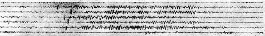
Scientists typically study brain activity during sleep using the electroencephalogram, or EEG, which measures brainwaves at the scalp. Starting in the mid 1930s, the sleep EEG was first studied by looking at the traces of brainwaves drawn on a paper tape by a machine. Many important features of sleep are still based on what people almost a century ago could most easily observe in the complex waveform traces. Even the latest machine learning and signal processing algorithms for detecting sleep waveforms are judged against their ability to recreate human observation. What then can we learn if we expand our notion of sleep brainwaves beyond what was historically easy to identify by eye?

eeg trace — An original paper tape trace of EEG from the 1930s, showing sleep spindles. (Loomis et al., 1935)

One particularly important set of sleep brainwave events are called sleep spindles. These spindles are short oscillation waveforms, usually lasting less than 1-2 seconds, that are linked to our ability to convert short-term memories to long-term memories. Changes in spindle activity have been linked with numerous disorders such as schizophrenia, autism, and Alzheimer’s disease, as well as with natural aging. Rather than looking for spindle activity according to the historical definition, we develop a new approach to automatically extract tens of thousands of short spindle-like transient oscillation waveform events from the EEG data throughout the entire night. This approach takes advantage of the fact that transient oscillations will looks like high-power regions in the spectrogram, which represent salient time-frequency peaks (TF-peaks) in the spectrogram.

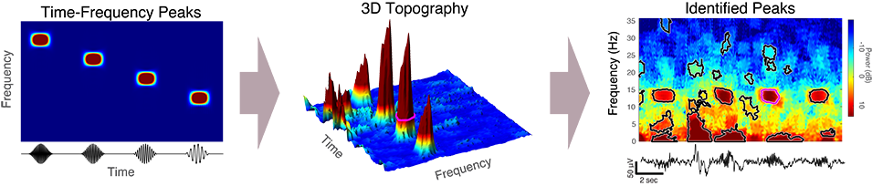
tf-peaks — Transient oscillation activity in the time domain will appear as contiguous high-power regions in the spectrogram, which represent salient peaks (TF-peaks) in the time-frequency topography.

The TF-peak detection method is based on the watershed algorithm, which is commonly used in computer vision applications to segment an image into distinct objects. The watershed method treats an image as a topography and identifies the catchment basins, that is, the troughs, into which water falling on the terrain would collect.

Next, instead of looking at the waveforms in terms of fixed sleep stages (i.e., Wake, REM, and non-REM stages 1-3) as di standard sleep studies, we can characterize the full continuum of gradual changes that occur in the brain during sleep. We use the slow oscillation power (SO-phase) as a metric of continuous depth of sleep, and slow-oscillation phase (SO-phase) to represent timing with respect to cortical up/down states. By characterizing TF-peak activity in terms of these two metrics, we can create graphical representations, called SO-power and SO-phase histograms. This creates a comprehensive representation of transient oscillation dynamics at different time scales, providing a highly informative new visualization technique and powerful basis for EEG phenotyping and biomarker identification in pathological states. To form the SO-power histogram, the central frequency of the TF-peak and SO-power at which the peak occurred are computed. Each TF-peak is then sorted into its corresponding 2D frequency x SO-power bin and the count in each bin is normalized by the total sleep time in that SO-power bin to obtain TF-peak density in each grid bin. The same process is used to form the SO-phase histograms except the SO-phase at the time of the TF-peak is used in place of SO-power, and each row is normalized by the total peak count in the row to create probability densities.

Quick Start

First, clone or download the MATLAB code for the toolbox from the main toolbox GitHub repository.

An example script is provided in the repository that takes an excerpt of a single channel of example sleep EEG data and runs the TF-peak detection watershed algorithm and the SO-power and SO-phase analyses, plotting the resulting hypnogram, spectrogram, TF-peak scatterplot, SO-power histogram, and SO-phase histogram (shown below).

Once the repository is cloned/downloaded, execute the example script on the command line:

> example_script;

Once a parallel pool has started (if applicable), the following result should be generated:

Output from the example segment of data provided with the toolbox.

This is the general output for the algorithm. On top is the hypnogram, EEG spectrogram, and the SO-power trace. In the middle is a scatter-plot of the TF-peaks with x = time, y = frequency, size = peak prominence, and color = SO-phase. On the bottom are the SO-power and SO-phase histograms.

Additionally, you should get a peak statistics table stats_table that has all of the detected peaks. The example script also creates stats_table_SOPH, which has the features for just the peaks used in the SO-power/phase histograms and is used for plotting.

These tables have the following features for each peak:

Feature	Description	Units
Area	Time-frequency area of peak	sec*Hz
BoundingBox	Bounding Box: (top-left, time top-left, freq, width, height)	(sec, Hz, sec, Hz)
HeightData	Height of all pixels within peak region	μV^2/Hz
Volume	Time-frequency volume of peak in s*μV^2	sec*μV^2
Boundaries	(time, frequency) of peak region boundary pixels	(seconds Hz)
PeakTime	Peak time based on weighted centroid	sec
PeakFrequency	Peak frequency based on weighted centroid	Hz
Height	Peak height above baseline	μV^2/Hz
Duration	Peak duration in seconds	sec
Bandwidth	Peak bandwidth in Hz	Hz
SegmentNum	Data segment number	#
PeakStage	Stage: 6 = Artifact, 5 = W, 4 = R, 3 = N1, 2 = N2, 1 = N3, 0 = Unknown	Stage #
SOpower	Slow-oscillation power at peak time	dB
SOphase	Slow-oscillation phase at peak time	rad

You can also look at an overview of the resultant peak data by typing the following in the command prompt (omit the semicolon to see output):

summary(stats_table)

Changing the Preset Time Range

Once the segment has successfully completed, you can run the full night of data by changing the following line in the example script under DATA SETTINGS, such that the variable data_range changes from ‘segment’ to ‘night’. ‘night‘;

%%Select 'segment' or 'night' for example data range
data_range = 'night';

This should produce the following output:

Changing the Quality Settings

The following preset settings are available in our example script under ALGORITHM SETTINGS. As all data are different, it is essential to verify equivalency before relying on a speed-optimized solution other than precision.

“precision”: Most accurate assessment of individual peak bounds and phase
“fast”: Faster approach, with accurate SO-power/phase histograms, minimal difference in phase
“draft”: Fastest approach. Good SO-power/phase histograms but with increased high-frequency peaks. Not recommended for assessment of individual peaks or precision phase estimation.

Adjust these by selecting the appropriate and changing quality_setting from ‘fast’ to the appropriate quality setting.

%Quality settings for the algorithm:
%   'precision': high res settings
%   'fast': speed-up with minimal impact on results *suggested*
%   'draft': faster speed-up with increased high frequency TF-peaks, 
%           *not recommended for analyzing SOphase quality_setting = 'draft';

Changing the SO-power Normalization

There are also multiple normalization schemes that can be used for the SO-power.

‘none’: No normalization. The unaltered SO-power in dB.
‘p5shift’: Percentile shifted. The Nth percentile of artifact free SO-power during sleep (non-wake) times is computed and subtracted. We use the 5th percentile by default, as it roughly corresponds with aligning subjects by N1 power. This is the recommended normalization for any multi-subject comparisons.
‘percent’: %SO-power. SO-power is scaled between 1st and 99th percentile of artifact free data during sleep (non-wake) times. This this only appropriate for within-night comparisons or when it is known all subjects reach the same stage of sleep.
‘proportional’: The ratio of slow to total SO-power.

To change this, change SOpower_norm_method to the appropriate value.

%Normalization setting for computing SO-power histogram:
%   'p5shift': Aligns at the 5th percentile, important for comparing across subjects
%   'percent': Scales between 1st and 99th ptile. Use percent only if subjects all reach stage 3
%   'proportion': ratio of SO-power to total power
%   'none': No normalization. Raw dB power
SOpower_norm_method = 'p5shift';

Saving Output

You can save the image output by adjusting these lines:

%Save figure image
save_output_image = false;
output_fname = [];

You can also save the raw data with by changing the value of save_peak_properties:

%Save peak property data
%   0: Does not save anything
%   1: Saves a subset of properties for each TFpeak 
%   2: Saves all properties for all peaks (including rejected noise peaks) 
save_peak_properties = 0;

Running Your Own Data

The main function to run is run_watershed_SOpowphase.m

run_watershed_SOpowphase(data, Fs, stage_times, stage_vals, 'time_range', time_range, 'quality_setting', 
                         quality_setting, 'SOpower_norm_method', SOpower_norm_method);

It uses the following basic inputs:

%       data (req):                [1xn] double - timeseries data to be analyzed
%       Fs (req):                  double - sampling frequency of data (Hz)
%       stage_times (req):         [1xm] double - timestamps of stage_vals
%       stage_vals (req):          [1xm] double - sleep stage values at eaach time in
%                                  stage_times. Note the staging convention: 0=unidentified, 1=N3,
%                                  2=N2, 3=N1, 4=REM, 5=WAKE
%       t_data (opt):              [1xn] double - timestamps for data. Default = (0:length(data)-1)/Fs;
%       time_range (opt):          [1x2] double - section of EEG to use in analysis
%                                  (seconds). Default = [0, max(t)]
%       stages_include (opt):      [1xp] double - which stages to include in the SOpower and
%                                  SOphase analyses. Default = [1,2,3,4]
%       SOpower_norm_method (opt): character - normalization method for SO-power

The main outputs are:

%       stats_table:   table - feature data for each TFpeak
%       SOpow_mat:    2D double - SO power histogram data
%       SOphase_mat:  2D double - SO phase histogram data
%       SOpow_bins:   1D double - SO power bin center values for dimension 1 of SOpow_mat
%       SOphase_bins: 1D double - SO phase bin center values for dimension
%                     1 of SOphase_mat
%       freq_bins:    1D double - frequency bin center values for dimension 2
%                     of SOpow_mat and SOphase_mat
%       spect:        2D double - spectrogram of data
%       stimes:       1D double - timestamp bin center values for dimension 2 of
%                     spect
%       sfreqs:       1D double - frequency bin center values for dimension 1 of
%                     spect
%       SOpower_norm: 1D double - normalized SO-power used to compute histogram
%       SOpow_times:  1D double - SO-power times

Algorithm Details

Time-Frequency Peak Detection

Spectral Estimation for Watershed Input

We use multitaper spectral analysis to estimate the time-frequency representation of the EEG signal, which acts is the input to the algorithm.

The following parameters are the default for the algorithm:

Data window: 1 sec, with 0.05 sec step size
Time-half-bandwidth: 2
Number of tapers: 3 tapers
NFFT: 2¹⁰
detrend: ‘constant’

This creates a spectrogram a spectral resolution of 4Hz. When computing SO-power and SO-phase histograms, peaks with frequency below 4Hz are not considered in the analysis since they cannot be disambiguated from the slow oscillation itself and may be contaminated by spectral leakage. The high NFFT provides an interpolation which allows for smooth TF-peak boundaries. The ‘constant’ detrend option sets each data window to be zero-mean.

These default parameters were chosen with the goal of optimizing the temporal/frequency resolution tradeoff in TF-peak detection, and to correspond with results from Dimitrov et al. in which TF-peaks have been shown to provide a more robust characterization of spindle-like activity than traditional spindle detection. While certain features such as TF-peak bandwidth and duration may be sensitive to spectral estimator and choice of parameters, the topographical centroid tends to be robust to spectral estimator and parameters.

See Prerau et. al 2017 and our tutorial pages on multitaper spectral estimation for detailed discussion of the theory behind multitaper spectral estimation, goals for principled parameter selection, and sleep EEG spectrogram dynamics. Our full multitaper spectral estimation package is available at https://github.com/preraulab/multitaper_toolbox

Watershed Procedure

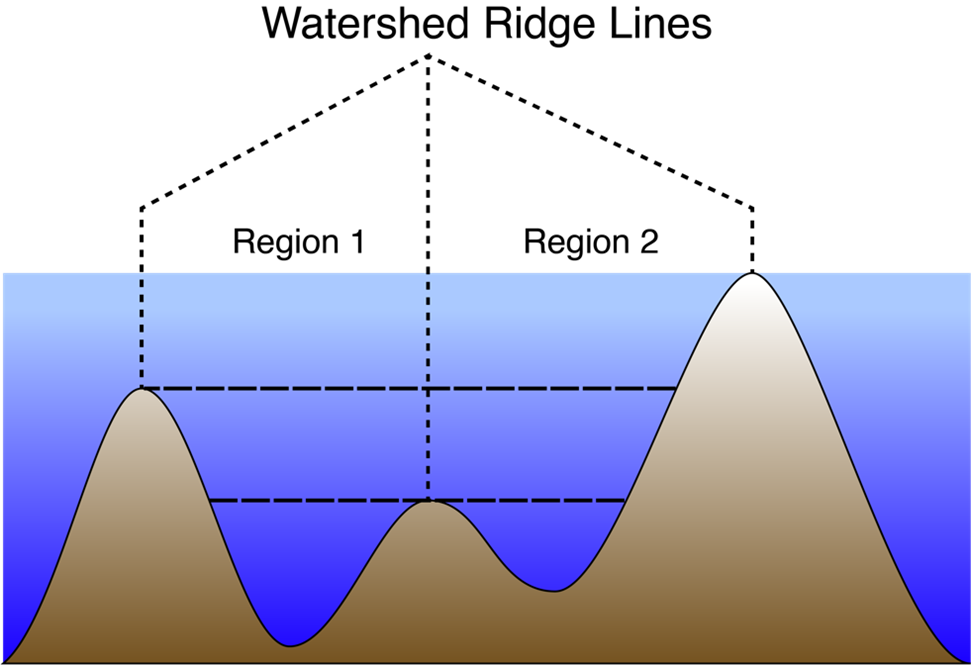
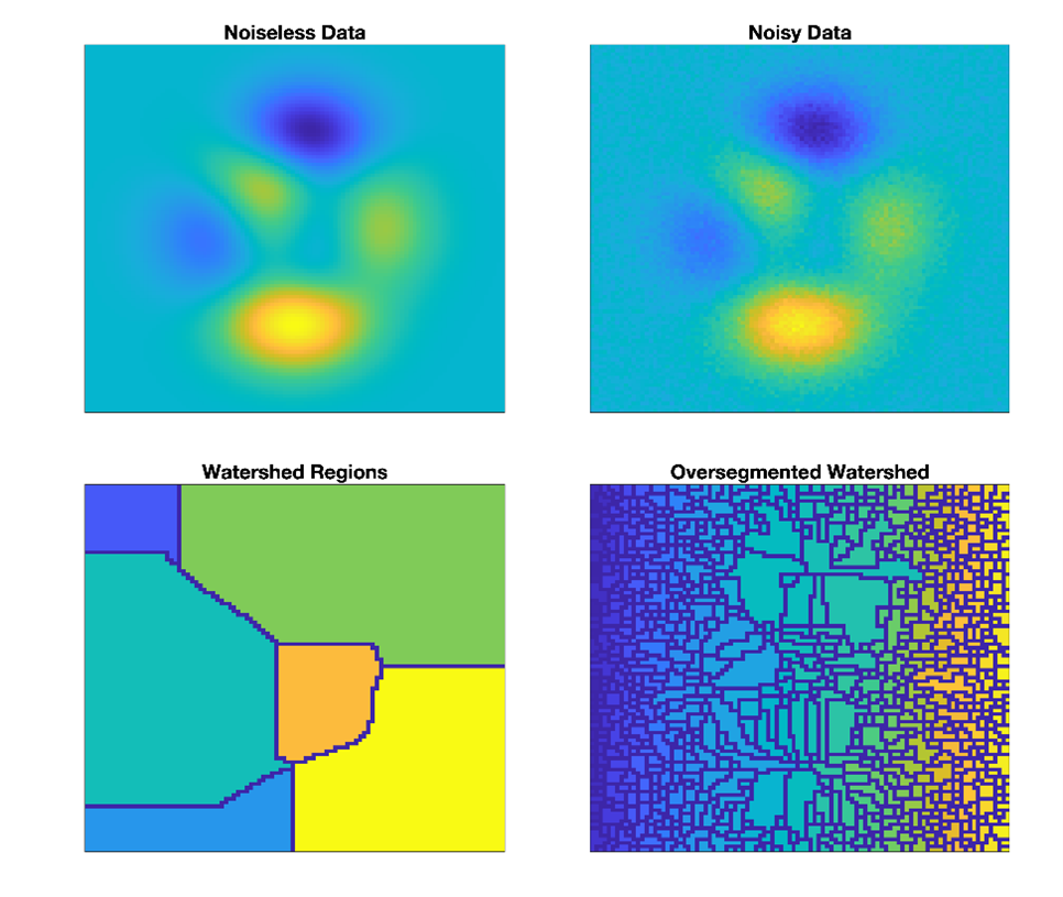
This approach is based on the watershed algorithm (Čomić et al., 2014; Kornilov & Safonov, 2018; Romero-Zaliz & Reinoso-Gordo, 2018), which is commonly used in computer vision applications to segment an image into distinct objects. The watershed method treats an image as a topography and identifies the catchment basins, that is, the troughs, into which water falling on the terrain would collect (Figure 1). We use the MATLAB implementation of the watershed, watershed(), which is based on the Fernand Meyer implementation (Meyer, 1994), to the negative of the baseline-normalized spectrogram in raw power units (not dB), thus identifying the local maxima and their surrounding regions.

Figure 1: The watershed algorithm identifies the catchment basins (regions) and ridge lines (dotted) in a topography by looking for points where a rising tide connects adjacent regions (dashed). As we wish to identify peaks instead of basins, we run the watershed on the negative topography.

Watershed Merge Procedure

Given noisy data, the watershed algorithm tends to over-segment the data, as noise produces lots of local extrema (Figure 2). To reduce over-segmentation, standard practice is for neighboring regions to be merged using a rule based on the specific needs of the application (Čomić et al., 2014; Kornilov & Safonov, 2018; Romero-Zaliz & Reinoso-Gordo, 2018). Here, for identifying transient oscillations, we developed a novel merge rule designed to form complete, distinct peaks in the spectrogram topography. By using the watershed as the basis for peak detection, we provide additional flexibility over previous methods (Dauwels et al., 2010; Olbrich et al., 2011; Olbrich & Achermann, 2005, 2008), which are based on parametric models of spectra or the spectrogram.

Figure 2: In perfectly smooth data, the watershed algorithm cleanly separates regions. However, the addition of even small amounts noise can greatly over-segments the data. We therefore require a procedure to merge over-segmented regions back together.

We develop a merge rule to combine create salient peaks with a large height relative to the base and surrounding boundary points of similar heights—but without overly merging distinct peaks. For this rule, we compute a weight between each watershed region and its neighbors, with a higher weight indicating a higher priority for merging.

For given watershed region $i$ , let $B_i$ be the heights of the pixels at the boundary between $i$ and all surrounding regions, and let $A_{i,j}$ be the heights at the adjoining boundary between region $i$ and neighbor $j$ . The merge weight between the two regions, $w_{i,j}$ , is based on two factors: $C_{i,j}$ and $D_{i,j}$ which are shown here.

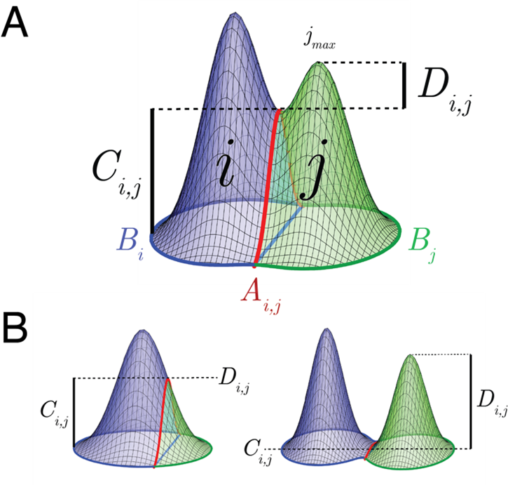Figure 3: Schematic of the weight computation for the watershed merge rule. (A) Given two regions $i$ and $j$ , we compute a directed weight for merging j into based on two factors: 1) $C_{i,j}$ – the difference between the max of the common border $A_{i,j}$ and the min of the border of region $i$ , $B_{i,j}$ , and 2) $D_{i,j}$ , the difference between the maximum of region $j$ and the maximum of $A_{i,j}$ . (A) These factors are indicative of the degree of separation and completeness of the two regions. (B) When a single peak is fractured (left), $D_{i,j}$ will tend to 0 leading to a high weight, and when peaks are separate (right), $C_{i,j}$ will tend to 0, leading to a low weight. We take the merge weight to be the maximum of the directed weights between the two regions.

When a peak is complete, we expect the boundary to be at similar heights all around, so we compute the difference between the maximum of the adjoining boundary pixels between region and and the overall minimum boundary point of region $i$ :

$C_{i,j}=max(A_{i,j}) - min⁡(B_i)$

The second factor relates to how distinct neighboring regions are from each other, and is the difference between $j_{max}$ , the maximum height of $j$ , and the maximum of the adjoining boundary:

$D_{i,j}= j_{max} - max⁡(A_{i,j})$

The overall directed weight, or importance to merge region into , is the difference between these factors:

$w_{i,j}=C_{i,j}-D_{i,j}$

Merging based on this weighting is specifically intended to prevent instances of large, contiguous peaks being fractured between two local maxima. The topographical components involved in the merge weights are illustrated in the above figure. In the general case (A), the difference between $C_{i,j}$ and $D_{i,j}$ is indicative of the degree of separation and completeness of the two regions. When a single peak is fractured (B, left), $D_{i,j}$ will tend to 0, leading to a high weight. When peaks are separate (B, right), $C_{i,j}$ will tend to 0, leading to a low weight.

Since the weights are directional, $w_{i,j} \ne w_{j,i}$ , so we take the undirected weight, $w^{i,j}$ , to be the maximum of $w_{i,j}$ and $w_{j,i}$

$w^{i,j}=max⁡(w_{i,j},w_{j,i})$

Following the initial watershed, the weights of all neighboring regions are computed. In an iterative manner, the regions corresponding to the largest weight are merged according to the corresponding direction. Any affected edge weights are then updated. This process continues until the largest weight is below a set threshold value. We use a threshold value of 8 based on preliminary empirical tests, but segmentation is qualitatively similar over a range of surrounding values. In practice, this acts as a hyper-parameter value that should be evaluated for each data set. Future work will explore means of optimizing the threshold value as well as possible alternative merge rules.

Peak Trimming

Given the properties of the watershed, our algorithm applied to a solitary peak on a flat surface will have bounds that go on forever. To compensate for peaks that lie on flat regions or other topographies that misrepresent the bounds of the peak, we define a volume-concentrated boundary, which contains 80% peak volume, and trim each region to this boundary. The boundary is identified by intersecting the peak topography with a plane such that the resulting boundary contains ≤ 80% of the original peak volume.

Noise Peak Removal

Most of the obtained peaks are due to un-merged local extrema, with small duration, bandwidth, and prominence, and thus likely to be noise. To account for this, we use the time and frequency resolutions of the spectrograms—the half-window length (0.5 sec) and half-bandwidth (2 Hz), as lower cutoffs. These cutoffs are features of the spectral estimator itself, which conservative limits that select peaks occurring at resolutions not possible to resolve given the estimator parameters. In addition, multitaper spectral estimation asymptotically follows a chi squared distribution. Thus, we use the lower bound of the 95% confidence interval based on the number of tapers used to add a peak height cutoff in the dB scale.

Estimation of TF-Peak Features

The time of each peak is determined by the weighted centroid of the trimmed region. Slow oscillation power and phase and sleep stage are determined for each peak based on the interpolated value at the peak time. In addition, we can compute TF-peak bandwidth, duration, area, prominence, maximum spectral power, and volume.

Computing SO-Power and SO-Phase Histograms

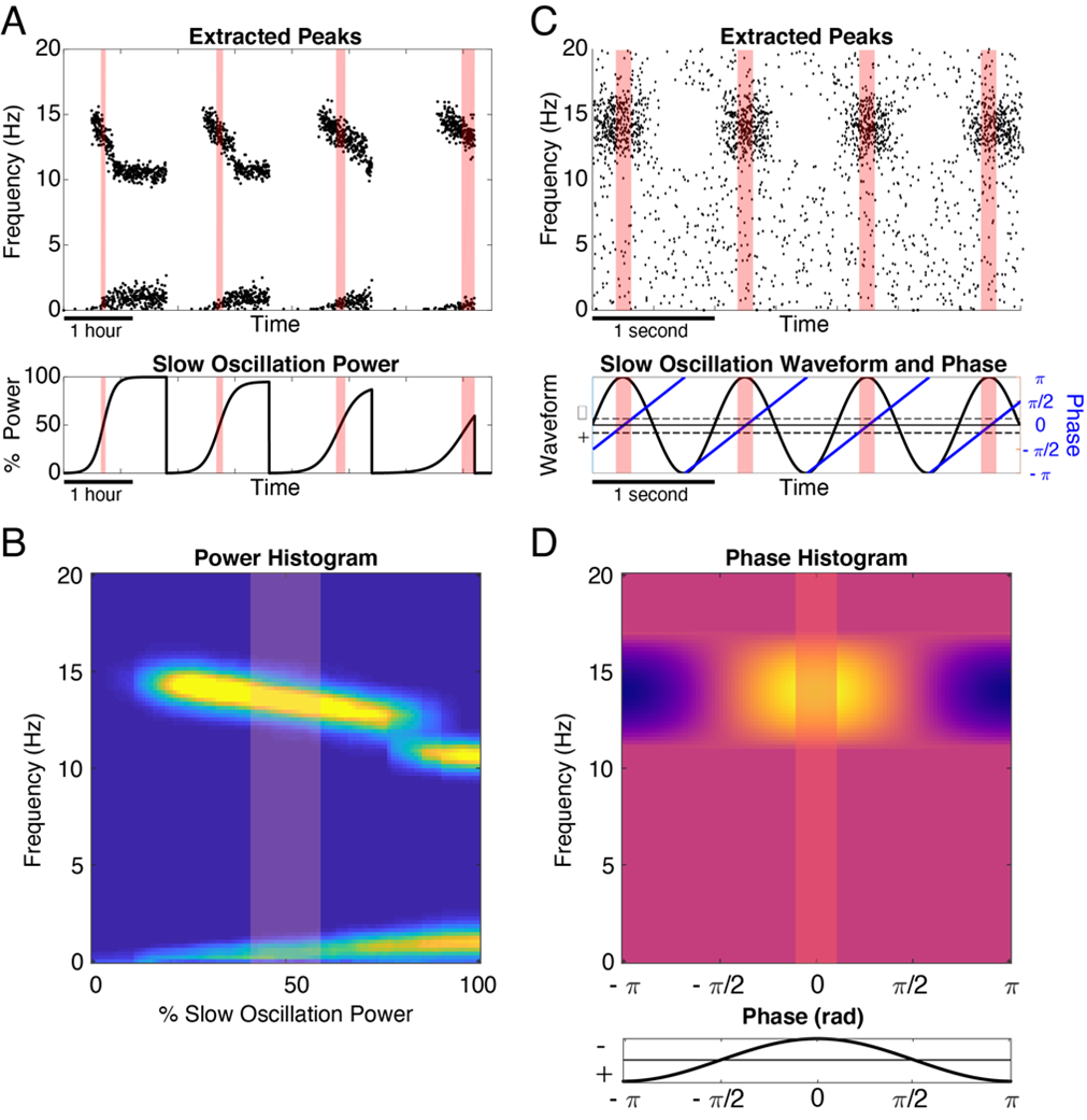
The SO-power histogram is a construct that allows us to observe patterns in TF-peak occurrence by looking at rate as a function of TF-peak central frequency and (0.3 to 1.5 Hz) SO-power. To form this two-dimensional histogram, we first create a matrix of discrete bins in frequency (rows) and bins in SO-power (columns). For all TF-peaks, we then extract the central frequency and SO-power at the time at which the peak occurred. We then create a two-dimensional histogram by counting the number of TF-peaks that fall into each frequency x SO-power bin. We convert the counts to a rate by normalizing each column by the amount of time spent within the corresponding SO-power for each bin. In Figure 4, A and B show a schematic of the basis for this histogram using simulated data.

The SO-phase histogram is a two-dimensional histogram analogous to the SO-power histogram but using TF-peak centroid frequency versus the SO-phase at the time of occurrence. Since phase is circular, we compute bins that wrap around +-π. In this case, we convert the TF-peak density to proportion by normalizing so that each row integrates to one. In Figure 4, C and D show a schematic of forming these histograms using simple simulated data.

SO Power and Phase Histogram calculation graphic

Figure 4: The construction of slow oscillation (SO) power and phase histograms. To characterize TF-peak density as function of depth of sleep and frequency, we can construct an SO-power histogram. (A) Given a set TF-peaks (upper panel) and %SO-power trace (lower panel) over time, we can construct a two-dimensional histogram by defining a set of frequency x %SO-power bins. We first find all the times in which %SO-power falls within a given bin. For example, red shaded regions in (A) and (B) represent a %SO-power bin of 40-60%. Each column of the SO-power histogram is then computed by taking the TF-peak count in each frequency bin divided by the total time the %SO-power fell within that bin. Similarly, we can characterize TF-peak phase coupling using an SO-phase histogram. (C) Given a set of TF-peaks (upper panel) and their corresponding SO-phase (lower panel, blue curve), we can compute a two-dimensional histogram using frequency x SO-phase bins. (D) We compute the SO-phase histogram by computing the density in the corresponding bins. As an example, red shaded regions in (C) and (D) represent a SO-phase bin of −π/8 to π/8. The densities are then normalized row-wise to get the proportion of activity within a given bin.

Slow-Oscillation Power

To estimate the slow-oscillation power (SO-power), we compute a second multitaper spectrogram with the following parameters:

Data window: 30 sec, with 15 sec step size
Time-half-bandwidth: 15
Number of tapers: 29 tapers

These parameters were selected to reflect the 30s stationarity assumption in ultradian dynamics implicit in traditional sleep scoring, while providing a 1Hz spectral resolution.

SO-power is computed by integrating between 0.3 to 1.5 Hz and converting to dB.

Slow Oscillation Normalization

The slow oscillation power can then be normalized with several approaches, with various benefits and limitations:

No normalization: The unaltered SO-power in dB.
Percentile shifted: The N^th percentile of artifact free SO-power during sleep (non-wake) times is computed and subtracted. We use the 5^th percentile by default, as it roughly corresponds with aligning subjects by N1 power. This is the recommended normalization for any multi-subject comparisons.
%SO-power: SO-power is scaled between 1^st and 99^th percentile of artifact free data during sleep (non-wake) times. This this only appropriate for within-night comparisons or when it is known all subjects reach the same stage of sleep.
Proportional: The ratio of slow to total SO-power.

TF-peak SO-power is computed by interpolating the normalized signal at the peak time.

Slow-Oscillation Phase

To estimate the slow-oscillation phase (SO-phase), the EEG time-domain signal is bandpassed from 0.3 to 1.5 Hz using a zero-phase filter approach. The filtered signal is then Hilbert transformed, and the angle extracted from the analy. TF-peak SO-phase is computed using interpolation of the unwrapped Hilbert phase at the TF-peak times. TF-peak phase was then re-wrapped such that a phase of 0 rad corresponds to the “peak” of the slow oscillation with respect to surface negative EEG, while a phase of π or −π rad corresponds to the “trough.”

Slow-Oscillation Power and Phase Histograms Construction

The generalized construction is summarized as follows:

Construction of a TF-Peak Feature Histogram

Given $P$ , a set of TF-peaks with a frequency and time, a feature signal (such as SO-power or SO-phase) $S_t$ , and a set of $M$ feature bins and $N$ frequency bins.

Define an $N \times M$ feature histogram, $FH_{(n,m)}$ .
For each feature bin, :
1. Find all times at which the signal $S_t$ falls within the given feature bin
2. Compute the total time $T_m$ for which $S_t$ fell within that bin.
3. For each frequency bin, :
  1. Define the rate within the feature spectrogram, $FH_{(n,m)}=|P_{(n,m)}|/T_m$ , where $P_{(n,m)}\subset P$ that fall into both the frequency and feature bin.

Implementation and Optimizations

Topographic Resampling

Perhaps the greatest computational load on this algorithm is performing the iterative merge procedure, the complexity of which is governed by segment size and resolution. To address this, use the following resampling approach for optimization:

Create a lower resolution spectrogram by downsampling the high-resolution spectrogram
Compute watershed and merge on the low-resolution spectrogram
Upsample the low-resolution merged regions to the resolution of the original high-resolution spectrogram
Use the boundaries of those regions and the data from the high-resolution spectrogram to trim peaks and to compute all peak statistics

In this way, we get rough estimates of the largest extent of the peaks, which are then refined by trimming in high-resolution. Overall, this approach provides great performance enhancements in the algorithm.

The consequence of downsampling, however, is that small adjacent noise peaks, which tend to occur at higher frequencies, may get joined together in the downsampling, thus falsely appearing to be a single larger peak with a false higher merge weight. To mitigate this issue, we can raise the merge threshold to reduce merging and retain a similar high frequency structure as the precision results.

Preset Settings

The following preset settings are available in our example script. As all data are different, it is essential to verify equivalency before relying on a speed-optimized solution other than precision.

“precision”: Most accurate assessment of individual peak bounds and phase
- 30s segments
- No resampling
- Merge threshold of 8
“fast”: Faster approach, with accurate SO-power/phase histograms, minimal difference in phase
- 30s segments
- 2×2 downsampling
- Merge threshold of 11
“draft”: Fastest approach. Good SO-power/phase histograms but with increased high-frequency peaks. Not recommended for assessment of individual peaks or precision phase estimation.
- 30s segments
- 1×5 downsampling
- Merge threshold of 13

Matlab Requirements

For the toolbox we currently require:

Signal Processing Toolbox
Image Processing Toolbox
Statistics and Machine Learning Toolbox

For parallel (optional)

Parallel Computing Toolbox
MATLAB Parallel Server

References

Čomić, L., De Floriani, L., Magillo, P., & Iuricich, F. (2014). Morphological modeling of terrains and volume data. Springer.

Dauwels, J., Vialatte, F., Musha, T., & Cichocki, A. (2010). A comparative study of synchrony measures for the early diagnosis of Alzheimer’s disease based on EEG. NeuroImage, 49(1), 668–693.

Dimitrov, T., He, M., Stickgold, R., & Prerau, M. J. (2021). Sleep spindles comprise a subset of a broader class of electroencephalogram events. Sleep, 44(9), zsab099. https://doi.org/10.1093/sleep/zsab099

Kornilov, A. S., & Safonov, I. V. (2018). An overview of watershed algorithm implementations in open source libraries. Journal of Imaging, 4(10), 123.

Loomis, A. L., Harvey, E. N., & Hobart, G. (1935). Potential Rhythms of the Cerebral Cortex During Sleep. Science, 81(2111), 597–598. https://doi.org/10.1126/science.81.2111.597

Meyer, F. (1994). Topographic distance and watershed lines. Signal Processing, 38(1), 113–125.

Olbrich, E., & Achermann, P. (2005). Analysis of oscillatory patterns in the human sleep EEG using a novel detection algorithm. Journal of Sleep Research, 14(4), 337–346. https://doi.org/10.1111/j.1365-2869.2005.00475.x

Olbrich, E., & Achermann, P. (2008). Analysis of the Temporal Organization of Sleep Spindles in the Human Sleep EEG Using a Phenomenological Modeling Approach. Journal of Biological Physics, 34(3), 241. https://doi.org/10.1007/s10867-008-9078-z

Olbrich, E., Claussen, J. C., & Achermann, P. (2011). The multiple time scales of sleep dynamics as a challenge for modelling the sleeping brain. Philosophical Transactions of the Royal Society A: Mathematical, Physical and Engineering Sciences, 369(1952), 3884–3901. https://doi.org/10.1098/rsta.2011.0082

Prerau, M. J., Brown, R. E., Bianchi, M. T., Ellenbogen, J. M., & Purdon, P. L. (2017). Sleep Neurophysiological Dynamics Through the Lens of Multitaper Spectral Analysis. Physiology, 32(1), 60–92. https://doi.org/10.1152/physiol.00062.2015

Romero-Zaliz, R., & Reinoso-Gordo, J. F. (2018). An Updated Review on Watershed Algorithms. In C. Cruz Corona (Ed.), Soft Computing for Sustainability Science (pp. 235–258). Springer International Publishing. https://doi.org/10.1007/978-3-319-62359-7_12