This toolbox can be used to compute an “instantaneous spindle rate” from sleep EEG data, quantifying moment-by-moment spindle regulation as a function of multiple simultaneous influencing factors.

Table of Contents

• Background and Toolbox Overview
• Quick Start
• Raw Data to Model Fitting
• Model Results and Visualizations
• Citations 

Sleep spindles are cortical electrical waveforms observed during sleep, considered critical for memory consolidation and sleep stability. Abnormalities in sleep spindles have been found in neuropsychiatric disorders and aging and suggested to contribute to functional deficits. Numerous studies have demonstrated that spindle activity dynamically and continuously evolves over time and is mediated by a variety of intrinsic and extrinsic factors including sleep stage, slow oscillation (SO) activity (0.5 – 1.5 Hz), and infraslow activity. Despite these known dynamics, the relative influences on the moment-to-moment likelihood of a spindle event occurring at a specific time are not well-characterized. Moreover, standard analyses almost universally report average spindle rate (known as spindle density) over fixed stages or time periods—thus ignoring timing patterns completely. Without a systematic characterization of spindle dynamics, our ability to identify biomarkers for aging and disordered conditions remains critically limited.

Using a rigorous statistical framework, we demonstrate that short-term timing patterns are the dominant determinant of spindle timing, whereas sleep depth, cortical up/down-state, and long-term (infraslow) pattern, features thought to be primary drivers of spindle occurrence, are less important. We also show that these short-term timing patterns are fingerprint-like and show increased variability over age. This study provides a new lens on spindle production mechanisms, which will allow studies of the role of spindle timing patterns in memory consolidation, aging, and disease.

Here, we provide this code toolbox to implement this integrated framework to characterizing instantaneous spindle temporal dynamics influenced by multiple factors, including sleep stage/depth (SO Power), cortical up/down states (SO Phase), and the past history of spindles. It consists of two major components:

• Load example data or upload their own data.
• Specify model factors and add interactions between them.
• Customize settings to generate an overview figure.

After installing the package, execute the “quick_start” GUI function in MATLAB command line to get started

> quick_start;

The following GUI should be generated (shown below, left panel):

Quick Start GUI

Let’s follow the 4 steps to make the choices. Here, we provide an example of the settings (shown above, right panel), which specifies the model we primarily used in the paper:

1. Load data: Load Example Data, which is the same MESA subject as in Figure 6 from the paper.
2. Select factors: Click on “Stage”, “SOphase”,”History”.
3. Choose history: Click on “Long-term (90 sec)”
4. Select interactions: Choose “stage:SOphase interaction”

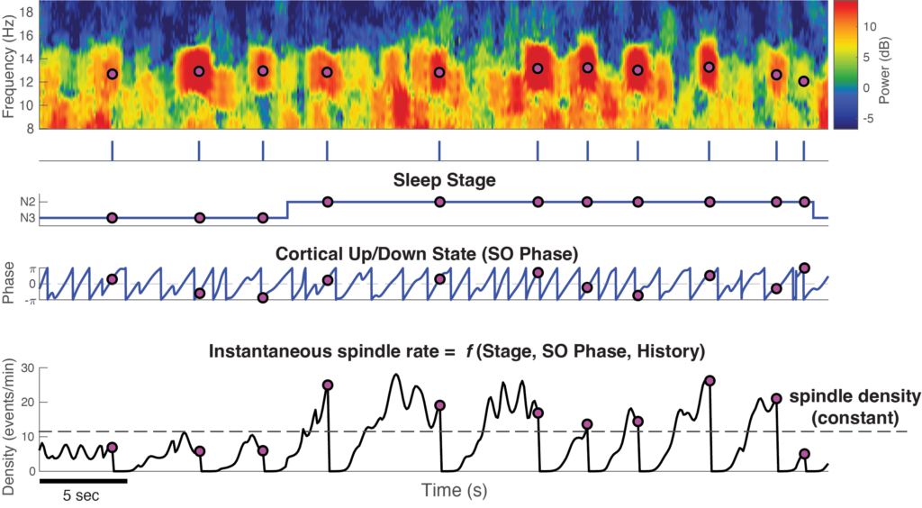
Once you clicked on “Run the Model” button, an overview figure will be generated for users to explore (shown below):

Overview of spindle dynamics

Use the scrollzoompan interface to slide and play around with the figure. To view the exact same epoch, set Zoom to be 90 and Pan to be 30145.

Click on “Load User Data”, it allows you to browse and load your own data. Ensure your data file meets the following requirements:

1. File format: The file must be a .mat file (MATLAB file format).
2. Required variables in the file: The .mat file must contain all the 4 variables (variable names are case-insensitive):
   • EEG: (double,1D vector) raw EEG data. Other accepted names: eeg_data, raw_EEG,data
   • Fs: (double,scalar) Sampling frequency of the EEG data in Hz. Other accepted names: sampling_rate
   • stage_val: (double,1D vector) Sleep stages(1: N3; 2: N2; 3:N1; 4:REM; 5:Wake). Other accepted names: stage_vals, stages,stage,stageval,stagevals
   • stage_time: (double,1D vector) Corresponding times for the sleep stages in sec. Other accepted names: stage_t, time_stages,stage_t,stage_times

In this section, we will walk through the data loading, preprocessing, model specification, and model fitting steps in the example script, highlighting the major functions. To run everything and generate all figures with a single command, simply execute the example script:

> example_script;

The specify_mdl consolidates all model specifications provided by users, including the model factors (BinarySelect), interactions to include(InteractSelect), and other additional options. These specifications are returned as a structured array (ModelSpec).

Usage:

[ModelSpec] = specify_mdl(BinarySelect,InteractSelect,'hist_choice',hist_choice,'control_pt',control_pt);

% Input:
%       <Required inputs>
%       - BinarySelect: (1x4 vector, double), indicates which factors are selected by the user
%         Factors are with fixed order: SOphase, stage, SOpower,history
%         e.g., [1,1,0,1] means select SOphase, stage, and history as model components 
%       - InteractSelect: (1xn cell), each entry contains an interaction term in the form of A:B 
%         It is case,order-insensitive, and accept multipler separators including:':', '&', and '-'
%         n is the number of interactions. For example, we can add 2 interactions
%         e.g., {'stage:SOphase', 'stage:history'} 
%
%       <Optional inputs>
%       - hist_choice: (string), it is either 'short'(default) or 'long'
%                   'short': Short term history (up to 15 secs, this option runs fast)
%                   'long': Long term history (up to 90 secs, use this to show infraslow structure)
%       - control_pt: (1xk vector,double), spline control point location, k is the number of control points
%                    default: [0:15:90 120 150]
%       - binsize: (double), point process bin size in sec, default: 0.1 sec
%       - hard_cutoffs:(1x2 vector,double), frequency cutoff in Hz
%                      default:[12 16], choose events in 12 to 16 Hz as fast spindles
%       
% Output:
%       ModelSpec: A struct that contains all model specifications

The preprocessToDesignMatrix function extracts spindle event information (res_table), saves preprocessed binned data (BinData), and design matrix (X) for model fitting.

Usage:

[X, BinData,res_table] = preprocessToDesignMatrix(EEG, Fs, stage_val, stage_time,ModelSpec);

% Input(All Required):
%       - EEG: (double, 1D), raw EEG data              
%       - Fs: (double, scalar), sampling frequency in Hz   
%       - stage_val: (double, 1D), stage values 
%                   where 1,2,3,4,5 represent N3,N2,N1,REM,and Wake
%       - stage_time:(double, 1D), corresponding time of the stage
%       - ModelSpec: A struct that contains all model specifications
%
% Output: 
%       - X (double, matrix): Design Matrix, the size depends on data length and ModelSpec
%       - BinData (struct): A struct that has all data saved in binsize 
%       - res_table: (table) All event info and signals to use. Key components include:
%           -- peak_ctimes: (cell), detected event central times (s)
%           -- peak_freqs: (cell), detected event frequency (Hz)
%           -- SOpow: (cell), slow oscillation power
%           -- SOphase: (cell), slow oscillation phase

In Matlab, glmfit function is applied to fit the point process – GLM model.

Usage:

[b, dev, stats] = glmfit(X,y,'poisson');

% Input:
%       - X: (double, matrix), design Matrix, the size depends on data length and ModelSpec
%       - y: (double, 1D), response, or point process binary train
%       - 'poisson': (string),  specified distribution 
%
% Output: 
%       - b: (double, 1D), fitted parameters
%       - dev: (double, scalar), deviance of the model
%       - stats: a Matlab struct that contains all the information of the model fitting result, including coefficient estimates (b), covariance matrix for b, p-values for b, residuals, etc.

In this section, we will walk through results part in the example script, highlighting the major functions.

The history modulation curve estimates a multiplicative modulation of the spindle event rate due to a prior event at any given time lag, which answers the question: How much more likely is there to be a spindle event, given that an event was observed X seconds ago? Using the plot_hist_curve.m function, we can plot the history modulation curve and save history features including refractory period, excitatory period, peak time, peak height, and infraslow multiplier.

Usage:

[xlag,yhat,yu,yl,hist_features] = plot_hist_curve(stats,ModelSpec,BinData)

% Input:
%       -stats (struct), results after model fitting 
%       -ModelSpec (struct), model specifications
%       -BinData, (struct), binned data
%
% Output:
%       -xlag (n x 1 vector), history time lag in sec
%       -yhat (n x k vector), history modulation value
%       -yu (n x k vector), history curve 95% confidence interval (upper)
%       -yl (n x k vector), history curve 95% confidence interval (lower)
%       Note: k = 1 when single history curve is computed
%             k = 2 when N2 and N3 history curve are computed, 
%               in which case, 1st col means N2 history, 2nd col means N3 history
%             n is determined by history lag and sp_resol (n = history lag in bin / sp_resol)
%       -hist_features (struct), it contains all history features, including
%          --ref_period: refractory period (s)
%          --exc_period: excited period(s)
%          --p_time: peak time (s)
%          --p_height: peak height
%          --AUC_is: The infraslow multiplier. Area under infraslow period (40s to 70s) / 30
%	-A history modulation figure

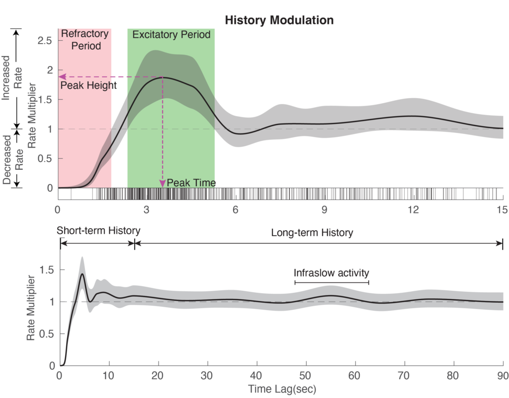Figure 1: History Modulation Curve

We observe that history modulation begins with a refractory period, during which spindles are less likely to occur. It then ramps up to a peak within an excitatory period, where spindle occurrence is most likely, before gradually decreasing back to 1, suggesting minimal modulation for events that occurred a long time ago. Here we show the Figure 2 in the paper for illustration purpose, but you can check the history curve for this example subject in the Overview of spindle dynamics figure.

2. Spindle Preferential SO Phase Shifts With Sleep Depth

Sleep spindles have been widely reported to preferentially occur in the cortical up state. Here we show the preferred phase shifts with sleep depth for this example subject. Use the plot_stage_prefphase.m function to visualize how preferred phase shifts with sleep stage.

Usage:

[pp,pp_CI] = plot_stage_prefphase(b,stats,ModelSpec)

% Input:
%       -b (double), fitted model parameters 
%       -stats (struct), all results after model fitting 
%       -ModelSpec (struct), model specifications
%
% Output:
%       -A figure that shows how preferred phase changes with sleep stage
%       -pp (3x1,double), preferred phase (rad) for N1, N2, and N3 stage
%       -pp_CI (3x2,double), 95% CI for preferred phase in N1, N2, and N3 stage
%                           1st column (lower bound for each stage)
%                           2nd column (upper bound for each stage)

Use the plot_sop_prefphase.m function to visualize how preferred phase shifts with with SOP (continuous sleep depth).

[phi0,sop0,sop_pp_mat] = plot_sop_prefphase(b,stats,ModelSpec)

% Input:
%       -b (double), fitted model parameters 
%       -stats (struct), all results after model fitting 
%       -ModelSpec (struct), model specifications
%
% Output:
%       -A figure that shows how preferred phase changes with continuous SOP
%       -phi0 (500x1, double), phase stamps for evaluation, 500 evenly spaced points from -pi to pi 
%       -sop0 (510x1,double), SOP stamps for evaluation, 510 evenly spaced points from -5 to 30
%       -sop_pp_mat (510x500 matrix,double), spindle rate heatmap as a function of (phi0,sop), 
%                                            in unit of events per binsize

Figure 2: Phase Shift: Stage vs. SO Power

We see spindles tend to occur in SO peak (phase ~0) during light sleep, and the preferred phase shifts earlier to the SO rising phase in deeper sleep, for this participant.

If the model is correct, the time-rescaling theorem can be used to remap the event times into a homogenous Poisson process. After rescaling, Kolmogorov-Smirnov (KS) plots can be used to compare the distribution of inter-spindle-intervals to those predicted by the model. A well-fit model will produce a KS plot that closely follows a 45-degree line and stays within its significance bounds (black). KS plots that are not contained in these bounds (red) suggest lack-of-fit in the model. Use the KSplot.m function to generate the KS plot, compute KS statistics, and output KS test results.

Usage:

[ks,ksT] = KSplot(CIF,y,ploton);

% Input:
%       - CIF (double), conditional intensity function
%       - y (double), binary event train
%       - ploton (double), output KS plot if ploton is 1 
% Output:
%       - A KS plot
%       - ks: KS statistic
%       - ksT: KS test result, 0 means pass the KS test
%                              1 means fail to pass the KS test

Figure 3: KS plot for models with different components

We observe that the model with the stage or phase factor does not pass the KS test. However, the model with a single history component passes the KS test, and the KS statistic is even smaller in the model with all factors.

The modeling framework allows us to quantitatively compare the relative contributions of these factors through deviance analysis, which is the point process equivalent of an analysis of model variance in linear regression. Use the compute_dev_exp.m function to compute proportional deviance explained by each factor.

Usage:

[dev_exp_sta,dev_exp_sop] = compute_dev_exp(BinData)

% Input: BinData (struct), all the binned data
%       
% Output: 
%       - dev_exp_sta (double,1x3), deviance explained from [stage, phase, history]
%       - dev_exp_sop (double,1x3), deviance explained from [SOP, phase, history]

Figure 4: Proportional Deviance Explained By Different Factors

From the table above, we see that the history component explains the most deviance, surpassing other factors such as sleep stage and SO phase.

The code contained in this repository is companion to the paper:

Shuqiang Chen, Mingjian He, Ritchie E. Brown, Uri T. Eden, and Michael J. Prerau*. Individualized temporal patterns drive human sleep spindle timing, Proc. Natl. Acad. Sci. U.S.A. 122 (2) e2405276121, https://doi.org/10.1073/pnas.2405276121 (2025).

which should be cited for all use.