This toolbox can be used to compute an “instantaneous AHI” from clinical sleep event data, providing individualized parameters that define the moment-to-moment probability of a respiratory event occurring.
Citation
Please cite the following paper when using this package:
Shuqiang Chen, Susan Redline, Uri T. Eden, and Michael J. Prerau. Dynamic Models of Obstructive Sleep Apnea Provide Robust Prediction of Respiratory Event Timing and a Statistical Framework for Phenotype Exploration, Sleep, 2022, zsac189, https://doi.org/10.1093/sleep/zsac189
Toolbox Code
Download the Apnea Dynamics Toolbox from our GitHub repository
Table of Contents
- General Information
- Data Format Description
- Building Design Matrix
- Model Fitting
- Model Visualization
- Example Data
General Information
Obstructive sleep apnea (OSA), in which breathing is reduced or ceased during sleep, affects at least 10% of the population and is associated with numerous comorbidities. Current clinical diagnostic approaches characterize severity and treatment eligibility using the average respiratory event rate over total sleep time (apnea hypopnea index, or AHI). This approach, however, does not characterize the time-varying and dynamic properties of respiratory events that can change as a function of body position, sleep stage, and previous respiratory event activity. Here, we develop a statistical model framework based on point process theory that characterizes the relative influences of all these factors on the moment-to-moment rate of event occurrence.
This model acts as a highly individualized respiratory fingerprint, which we show can accurately predict the precise timing of future events. We also demonstrate robust model differences in age, sex, and race across a large population. Overall, this approach provides a substantial advancement in OSA characterization for individuals and populations, with the potential for improved patient phenotyping and outcome prediction.
In this tutorial, we provide the corresponding codes to walk through people step by step, from model input construction to model fitting, model visualization, and model goodness-of-fit.
Data Format Description
In general, to analyze apnea dynamics, we need these required information: the apnea event end times, sleep stage times and corresponding stages, position times and corresponding positions. In the example data, the data file that contains all these information is saved in .mat (Matlab) forms, where each subject has an individual struct file that includes:
- AHI: Apnea Hypopnea Index, in events/hour
- N: Total number of respiratory events
- TST: Total sleep time, in hours
- event_info: [3 x N], double, respiratory events information, [event_start_time, event_duration, event_type]
- event_type:
- 1: hypopnea
- 2: obstructive event
- 3: central event
- event_type:
- hypnogram: [H x 3], double, sleep stage information, [stage_start_time, stage_duration, corresponding_stages], for corresponding_stages
- 1: N3 stage
- 2: N2 stage
- 3: N1 stage
- 4: REM (Rapid Eye Movement sleep)
- 5: Wake
- rawposition: [P x 1], vector, double, sleep positions recorded in sampling frequency Fs_pos, which is 32 Hz in MESA dataset. 0:Right; 1: Back; 2: Left; 3: Prone; 4: Upright, which in our implementation, will be relabeled as:
- 1: Supine (Sleep on back)
- 0: Non-Supine (Right, Left, Prone, Upright)
Building Design Matrix
To prepare for the model fitting, we need to convert the data into a design matrix that contains all the predictors and a corresponding response column that indicates the apnea event occurrence. Apnea event times were discretized into 1-second intervals and the time series the number of respiratory events (0 or 1) terminating in each of those intervals was computed.
- Response (y): [n x 1] vector, binary (0 or 1) event train, 1 means the apnea event happened at that time interval
- Design matrix: [n x 15] matrix defined as [pos sta history]
- Body position (pos): [n x 1] vector, binary (0 or 1), 1 means Supine position at that time interval
- Sleep stage (sta): [n x 5] matrix defined as [N1 N2 N3 REM Wake], binary (0 or 1), value 1 in each stage column indicates the corresponding stage the participant is in at that time interval
- Event history (history):[n x 9] matrix describes the past event activity in the cardinal spline basis
- Total time lag: 150
- Tension parameter s: 0.5
- Number of knots: 9
- Knot location setting: With end points at 0 and 150 seconds, 4 knots were placed evenly between the 10th percentile of inter-event intervals and 90 seconds, with another knot at 120 seconds. Two additional knots placed at -10 and 160 seconds were used to determine the derivatives of the spline function at the end points
- Other data saved:
- Sp: [ord x 9] double, cardinal spline matrix
- isis: [, x 1] double, inter-event-intervals in seconds
The function build_design_mx.m is provided to reformat the saved data so they are used to build design matrix and response for model fitting.
Usage:
[pos,sta,history,y,Sp,isis] = build_design_mx(bin,Fs_pos,ord,event_info,hypnogram,rawposition)
Model Fitting
In Matlab, glmfit function is applied to fit the point process-GLM model.
- Input:
- Design matrix: [pos sta history]
- Response: y
- Specify distribution: ‘poisson’
- Include constant or not: ‘constant’, ‘off’
- Output:
- b: fitted parameters
- dev: deviance of the model
- stats: a Matlab struct that contains all the information about the model fitting result, including coefficient estimates (b), covariance matrix for b, p-values for b, residuals, etc.
Usage:
[b, dev, stats] = glmfit([pos sta history], y, 'poisson', 'constant', 'off');
Model Visualization
To compute the predicted values for the GLM, glmval function is applied
- Input:
- Fitted parameters: b
- Sp: the cardinal spline matrix
- link function: ‘log’
- stats: Matlab struct from the output of glmfit
- Include constant or not: ‘constant’, ‘off’
- Output:
- yhat: [150 x 1] vector, history dependence curve
- ylo: yhat – ylo defines the 95% lower confidence bound of yhat
- yhi: yhat + yhi defines the 95% upper confidence bound of yhat
Usage:
[yhat,ylo,yhi] = glmval(b,[zeros(150,6) Sp],'log',stats,'constant','off');
Example Data
We apply the modeling approach to several example subjects from MESA dataset (the same subjects as the Figure 1 B&C in the paper), they have similar AHI (~ 30 events/hr) but very different event patterns. For a single subject, example1_script.m is provided in the repository to load the sample data, convert to the design matrix, run the model, output the results, generate history curves as well as goodness-of-fit.
Step 0: Load saved data
First, we load a single subject from MESA dataset that contains all the information we need (see details in the Data Format Description section).
%% Load data for a single subject
load('Example_data/example1sub.mat');

%% Pre settings
bin = 1;                                     % set bin size (seconds)
Fs_pos = 32;                                 % sampling freq for position in MESA dataset
ord = 150;                                   % total number of orders we consider in history
AHI = sub2127.AHI;                           % AHI in events/hr
N = sub2127.N;                               % Number of respiratory events
TST = sub2127.TST;                           % Total Sleep Time in hours
We then set up the variables we need to build the design matrix
Step 1: Build and visualize design matrix & response
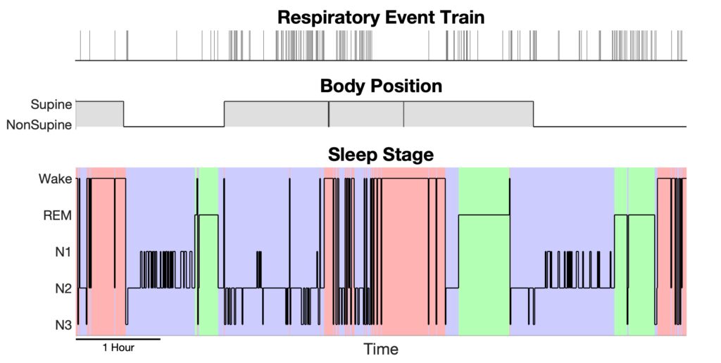
After we perform the function build_design_mx.m to reformat the saved data into a design matrix and the corresponding response, we can visualize them using plot_DesignMx_Resp.m function.
%% - Step 1: Convert saved data to design matrix and response

[pos,sta,history,y,Sp,isis] = build_design_mx(bin,Fs_pos,ord,sub2127.event_info,sub2127.hypnogram,sub2127.rawposition);

%% -- Step 1+ : Visualize the position, stage and event train

plot_DesignMx_Resp(pos,sta,y);
Step 2: Fit model and output result
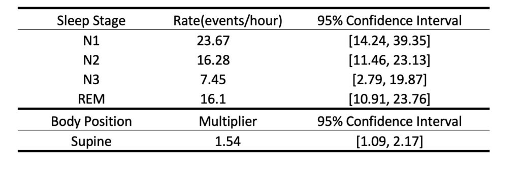
Based on the design matrix and response, we can run the model using MATLAB built-in function glmfit. We can summarize the fitted parameters as an output table to show the event rates in different sleep stages and a supine multiplier, as well as their 95% confidence intervals. The functionsave_output_tbl.m will report an output table as shown below and save it as a .csv file to your current folder.
%% - Step 2: Model fitting

[b, dev, stats] = glmfit([pos sta history],y,'poisson','constant','off');

%% -- Step 2+: Visualize model output as a table

[tbl] = save_output_tbl(bin,b,stats)
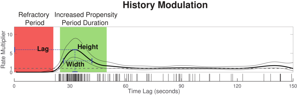
Step 3: Plot history modulation curve
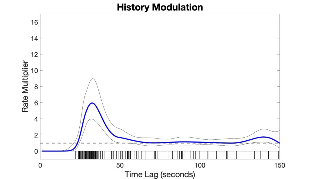
The history modulation curve estimates a multiplicative modulation of the event rate due to a prior event at any given time lag, which answers the question: How much more likely is there to be a respiratory event, given that an event was observed X seconds ago? Use the plot_hist_mod_curve.m function to generate the history modulation curve.
%% - Step 3: Plot history modulation curve
[yhat,ylo,yhi] = glmval(b,[zeros(ord,6) Sp],'log',stats,'constant','off');

% 95% Confidence bounds for history curve
hi_bound = yhat + yhi;
lo_bound = yhat - ylo;

% Figure
plot_hist_mod_curve(bin,ord,yhat,lo_bound,hi_bound,isis);
Step 5: Evaluate model goodness-of-fit using KS plot
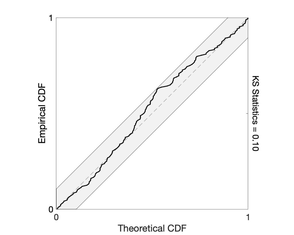
If the model is correct, the time-rescaling theorem can be used to remap the event times into a homogenous Poisson process. After rescaling, Kolmogorov-Smirnov (KS) plots can be used to compare the distribution of inter-event times to those predicted by the model. A well-fit model will produce a KS plot that closely follows a 45-degree line and stays within its significance bounds. KS plots that are not contained in these bounds suggest lack-of-fit in the model. Use the ks_plot.m function to generate the KS plot.
%% - Step 4: Evaluating model goodness-of-fit using KS plot

[ks,ksT] = ks_plot(pos,sta,history,y,b);
Nearly same AHI, dramatically different history modulation structures
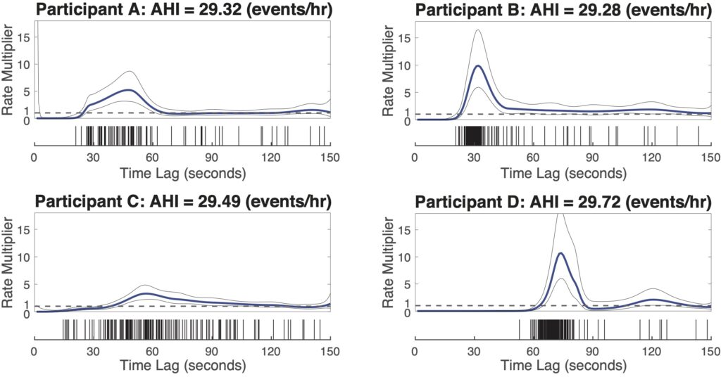
Here, we show four example subjects from MESA dataset, with similar AHI (~ 30 events/hr) but different history modulation curves. The script, example4_script.m is provided to generate the following figure.
Adding history component to the framework allows us to capture the dynamic patterns of the respiratory events and greatly improve our predictability in the event timings. These dynamic patterns act as individualized respiratory fingerprints, providing the potential to phenotype patients, and to personalize therapeutic approaches by controlling airway pressure in a dynamic fashion based on moment-to-moment prediction of respiratory events.